Excursion: the impact of climate change on Heterodera schachtii populations

How growth processes of both nematode and host might change with temperature increase?

This background page of the HS-project provides some more detailed information about Heterodera schachtii and Climate change based on temperature data from 1902 to 2100 for a sugar beet production area in the Rhineland, Germany.

1. Stage dynamics of H. schachtii

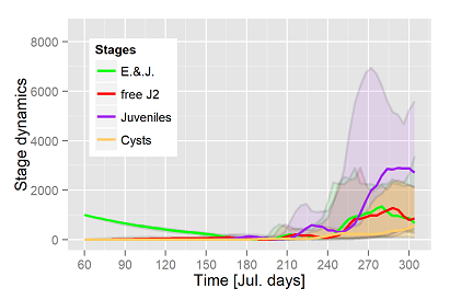
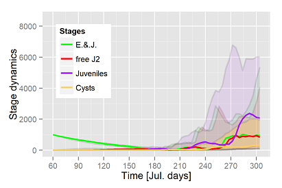
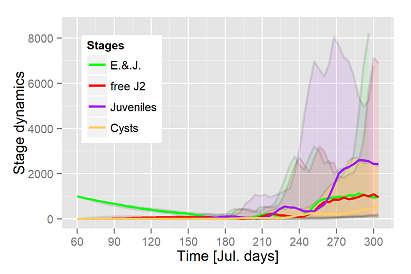
Stadienentwicklung von Heterodera schachtii — Fig. 1a: Simulated stage dynamics 1902-2000

Dynamics of nematode stages — Fig. 1a: Simulated stage dynamics 1902-2000

No accelerated development processes are detected on the first view. The slow juvenile development of the host maintains in all four periods. Just beyond 2050 (!) the appearance rate of the juveniles might be earlier, not in the mean, but as seen in the 5% quantile. As shown in the variance extreme events occur more often in the 21^st century than in the last century.

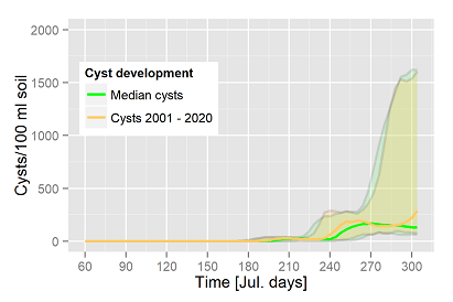
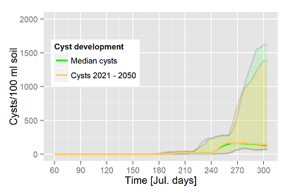
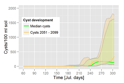
Cysts development of Heterodera schachtii — Fig. 2a: Simulated cysts dynamics 1902-2000

The cysts dynamics of the single periods (P1-P4) are compared to the overall median (incl. confidence area) of 200 years in fig. 2 a-d. The variance show both the change on the time axis and population changes on the y-axis. No matter which period is of concern, a mean cysts population is build up at the end of the season. It ranges from 150-200 cysts/100 ml soil (green line). A small delay is shown in the beginning of P1 compared to the overall mean, the top cyst increases are below the extremes, but occasionally new cysts densities of more than 800 are produced. With respect to the variance P2 represents more or less the overall mean, but in the end more cysts are produced on average (yellow line, fig. 3b). More extreme events happens in P2. The system "calms down" a little bit through the 3^rd period, extremes continue to occur, but less frequent than in P2. The system accelerates again in P4. Cysts show up earlier in the extremes and exceed the mean top values. On average the cysts numbers increase significantly.

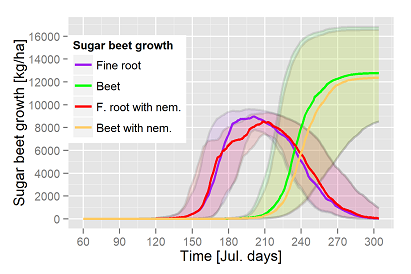
2. Compared yield structures of the sugar beet

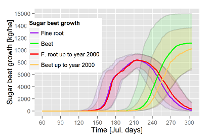
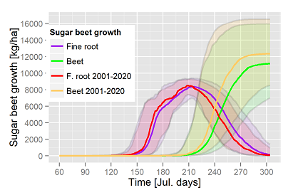
Sugar beet growth — Fig. 3a: Simulated sugar beet growth 1902-2000

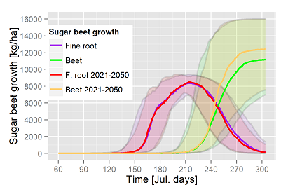
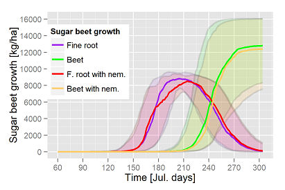
Again the results of each period is compared to the overall median including variance. The dynamics of the compartment "Fine root" define the habitat of the nematode in terms of volume and time. The growth period is prolonged in P1 compared to the overall mean, beet growth is slightly delayed, the total growth period of the beet is shortened and yields are lower than the common mean. 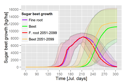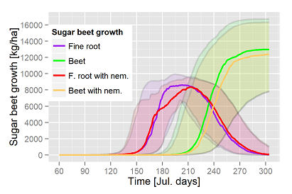Growth dynamics are slightly accelerated in P2, yields are above average, variation as well. P3 relates approximately the mean dynamics, yields are similar to P2. The dynamics are getting faster in P4, yields increase further. Yield prediction is just a minor outcome of modeling H. schachtii, hence first the absolute yields must be seen in relation to each other and second there are no yield restrictions within the model equations, which might causes yield limits at higher temperatures, as for example potential drought periods in P4.
But, most interesting, the simulated yield potential of the time periods are related to changing temperatures only, and not to improved varieties, production technology or similar.

2. Yield/loss relation

Another but secondary question: How are the yield/loss relations changing at given Pi of 1000 E&J/100 ml soil and increasing temperatures? The usual graphical summary follows in fig. 4.

Yield/losses with H. schachtii — Fig. 4a: Yield/loss relation 1902-2000

The relative differences are marginal, in P1 varies the (numerical) loss rate in the range of 1 to 5%, in P2 and 4 around 2%, just in P3 are 9% predicted in one of the worse scenarios. No trend is seen with time.