Further explanation for the use and interpretation of canonical distances
Summary
The canonical distance provides a measure of a quantitative comparison of
different experimental designs, condense the test conditions and define the
intensity of treatment factors on a dimensionless scale. As larger this value as
larger the differences and therefore the treatment effect.
The canonical distances are the main focus of our techniques concerning the
quantitative analysis of hyperspectral signatures.
The canonical distances are the
result of a cascade of statistical procedures in terms of model
fitting and multivariate statistics. They describe the average
vectors within the discriminant area or space obtained from the
discriminant scores of the spectra.
Why is this value most interesting?
This dimensionless value quantifies the difference between two or more
traits or classes of traits. It demonstrates the relative difference between
two traits as an universal number over all treatments. The spectra contain
information about both the experimental design as well as the standard
number for the experimental run. Similar to a multiple mean comparison test
the distance addresses the absolute size of the treatment effect in terms of
the length of the arrow. Distances larger than 2 generally give evidence for
a significant difference (varies with the variance). Additionally the
variance is observable and open for related interpretations.
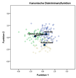
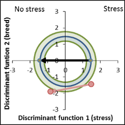
Fig 1: Canonical distances of vine leaf pathogens
Example of pathogens on vine leaves, fig. 1,
measurements were taken before any symptoms have been visible: The
distance between downy mildew (P. viticola) infected plants
and the control is above 3, which is a significant value. In
contrast the figure shows the position of another pathogen, black
rot (G. bidiwellii), again before symptoms have been
noticed. Also the distance is significant, but smaller than compared
to P. viticola. The inoculated plants are suffering from a stress (pathogen) and
the distances determine the degree of stress.
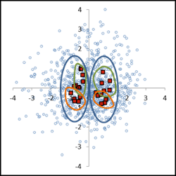
Fig. 2: Analysis of multifactorial experiments Interpretation of a multifactor experiment (fig. 2):
The first factor (blue area) is most distinguishable. The dominance is interfering with the two other factors.
Inside the 2nd factor (green area) as well the 3rd factor (orange area) are no differences,
the related distances are too small. Discussing a tendency, factor 2
and 3 are slightly different, the
distances approaching the boundaries of decision making, but the distances are below the significance limit.
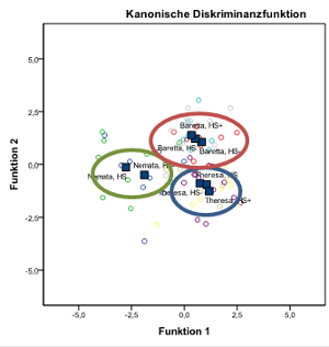
Fig 3: Impact of nematodes and variety effect
Interpretation of a two way experiment: The 1st factor
(variety) shows most obvious a discrimination, the boundaries of the variety are clear, the 2nd factor (nematode population density)
is not different. The distances within a group are just marginal. An allocation to population density classes (low, medium, high)
is not possible.
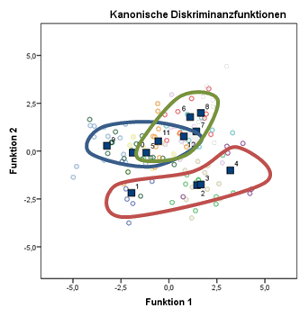
Fig 4: Impact of nematodes and variety effect with predetermined density classes
Same experiment as before, different year, presented in
12 combined classes with interaction. The existing nematode population are partitioned in four classes (low, medium, high, very high)
and linked to the varieties (1-4 susceptible variety; 5-8, resistant variety; 9-12, tolerant variety).
The hyperspectral measurements from the sugar beet canopy allow conclusion about the nematode density
dependent on the variety characteristics. The susceptible variety is stronger affected by the
nematode, while the nematode effect is not that clear for the tolerant / resistant varieties.
Fig 5: Trait regcognition on canonical distance spaces and vector rotation
Rotating the vectors within the area
helps to discriminate the second factor visually out of large
sets of data. The vector of the control is set to a zero base line,
all other distances are corrected and compared with respect to
length and position within the discriminant area. The example is
used to differentiate traits of new varieties from hyperspectral
signatures. We can construct a confidence circle within the
discriminant area. The vectors of new varieties inside the circle
are not different from the traits of the control variety. Lines far
out of the circle are significant different from the control, but do
not satisfy the breeding objectives, the genetic distance is too
large. Most interesting for the further breeding program are lines
with vectors just touching the confidence circle and lengths below the control.
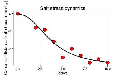
Fig. 6:Time series of hyperspectral measurements, ex. salt stress progress
The advantage of non-invasive sensors
include the ability for "endless" repeated measurements of the same
object. The dynamics of experiments are clearly shown by the
canonical distances (y-axis) put on the time axis. The example
demonstrates the effect of salt stress. The vary distances over
time are fitted to a logistic function and present the dynamics of
an increasing stress.
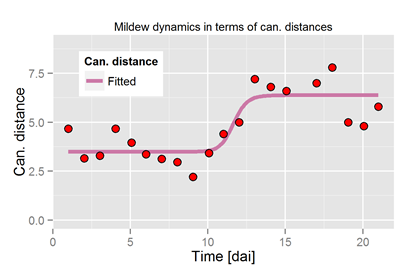
Fig. 7: Time series of hyperspectral measurements, ex. mildew disease progress
Disease progress in terms of canonical distances. Canonical score values cannot
always be transfered 1:1 to known situations. Disease progress follows mostly exponential processes.
On the scales of canonical distances a logistic model is appropriate. The systems detect
pathogen infection earlier, but approaches an upper saturation or asymptote earlier than the real disease.
Nemaplot uses cookies to provide its services. By continuing to browse the site you are agreeing to our use of cookies.
More information (in German only)