Multi factorial experiments

Case study 4: Factorial experiments

Hyperspectral measurements are most suitable for even more complex experimental designs. Based on the canonical distance advanced interpretation of multiple factors and factor levels are possible. We introduce a variety experiment (greenhouse pot experiment) of wine cultivars as an example. The following design was established: factor one variety with three levels. Used cultivars have been Müller-Thurgau (MT, susceptible), Regent (RE, resistant), Solaris (SO, resistant) ¹) and the factor disease (two levels: healthy/infected) with downy mildew, Plasmopara viticola, to test the response of the three varieties with respect to the fungi-like pathogen. The plants were inoculated by usual standard procedures at the beginning of the experiment. The used cultivars differ with respect to their degree of tolerance/resistance but also with respect to their leaf phenology. The experiment lasted for 12 days, reflectance measurements started 3 after inoculation. Measurements were taken from the three top leaves on the leaf surface in daily intervals.².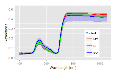

Durchschnittlicher Spektralvergleich von 3 Rebensorten — Fig. 1: Score-distribution after 12 days

Reflexion der Rebensorten mit P. viticola Infektion — Fig. 1: Score-distribution after 12 days

Effect of pathogen, variety and interaction — Fig. 3: Score-distribution after 12 days

Results

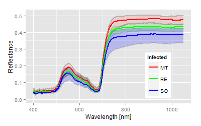
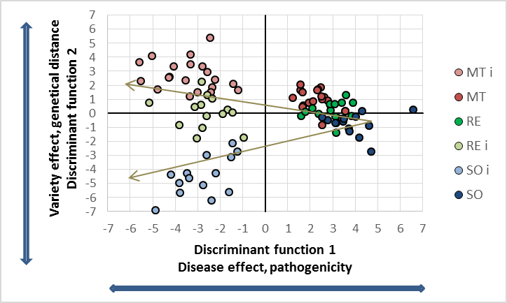
The significance of all statistical parameters is high, therefore we are stressing only the canonical distances as the degree of treatment differences. The used varieties show obvious reflectance differences in the control, the leaves of the cultivar Solaris are most different from the phenology (blue line in top figure left) compared to the other two varieties. The genetically differences increased drastically with the P. viticola infection (top figure right). The score distribution of the canonical area highlights both the pathogenicity of the pathogen on the x-axis and the variety specific (genetically) response with respect to given pathogenicity on the y-axis. As expected, all cultivars respond different to the infection and as seen in the relative relation within the canonical area. From the reflectance data no information can be given about the type of response. In fact the cultivar MT showed major tissue damages (as seen in the spectral pattern), while the variety RE and SO show the different resistance mechanism against P. viticola. The virtual expansion path defines the genetically characteristics in both without and with infection as well as the pathogenicity of the used inoculum.

Interaction and multiple mean comparison based on canonical distances

Strong treatment interaction can be noticed in this experiment. Mean comparison has to be restricted in this case. The following comparisons are possible in this case: a) infection combination x all cultivars (as depicted in the figure above), b) each cultivar x pathogen (relates to the x-axis of the graph, and c) comparison of each cultivar for each level of factor two, i.e. infected and uninfected (relates to y-axis of the graph. The following table summarises the mean distances of each legitimate combination.

Average canonical distances of potential mean comparisons
Combination a, all factor levels	Distance	Combination b, Pathogenicity of the inoculum	Distance	Combination c, genetically differences	Distance
MT x downy mildew	6.1	MT	7.6	MT vs. RE, control	0.83
RE x downy mildew	5.6	RE	12.1	MT vs. SO, control	2.24
SO x downy mildew	7.7	SO	9.5	RE-SO, control	1.42
				MT vs. RE, with pathogen	2.72
				MT vs. SO, with pathogen	7.23
				RE vs. SO, with pathogen	4.59

The mean canonical distances are extremely high in all cases, applying the usual criteria a value of 2 to 3 would be highly significant already. Those common result are exceeded widely. The graphical score distribution represents the mean comparison of combination a, the distances varies from 5 to 8. Apply the discriminant analysis solely for each variety, apparently increases the biotic stress, as the interaction is excluded. The result does not give evidence of yield losses or similar, or the cultivar is most affected by P. viticola, but a relative ratio of the specific varieties with respect to the intensity of the biotic stress. Combination C is most interesting: the genetically distances are determining the neighbouring similarity among the varieties. Solaris is most different from MT variety, the distance increases with the infection.

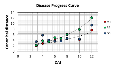
Disease progress curve base on canonical distances — Fig. 4: Disease progess curves in terms of hyperspectral signature

The experiment represents a time series of measurements. As we gain a canonical distance for each day representing the dynamics of P. viticola. The distances vary exponential with MT and RE, while the distances are different on SO. A high value of 4 is found at the beginning (in conclusion: SO has already responded to the infection)and does not change until the last day. The pathogen get encapsulated, so changes occur until day 10, but the pathogenicity of the inoculum overwhelmed the resistance of the host.

The trials have been repeated twice with a much lower inocula densities and different incubation conditions. Follow the link Analysis of multiple spectra with two factors

Please follow the additional link for another example of threefactorial designs in field salad

Summary

The ANOVA tables are not shown here, as high significances showed up instantly from the beginning of the measurements. The heterogeneity of the used cultivars or leaf age might have caused the differences in the beginning, not the infection. These differences can be observed in the mean spectra. Solaris generates a complete different spectrum in the untreated control (blue line) compared to the other two.
The quantitative analysis by the canonical distances provides an accurate description of the experimental situation and results.
The extremely high distance values does not give any conclusions about crop losses or similar responses. It just demonstrates how much "effort" is needed by the individual variety to handle this enormous pathogenicity of the pathogen.
Compared to similar follow up experiments with a much weaker pathogenicity we can see here how P. viticola has broken the resistance of the cultivars MT and SO in this experiment.
Using the given cultivars with well known resistance properties as standards, a new breed or line could be compared to the standards by its relative position on the discriminant area. Addressing both the similarity in terms of scores without biotic stresses as well as relative to the scale of the controlling parameter "pathogenicity" is possible. Derived from the experiment, the discriminant functions get a biological meaning.

More complex experimental designs include the advantage to account for interaction effects. The intensity of interaction can be described by the angle of centroids, but the interpretation of the angles are vague in the moment, as the rotation of the vectors varies with each measurement. Especially in plant breeding experiments a large number of new lines are compared to a control ( = standard cultivar). It is recommended to set the control parallel to x-axis and rotate all scores of the breeding lines with respect to the control or standard cultivar.

¹ Cultivars have been provided by the JKI Geilweiler Hof, Germany
² In cooperation with Privat-Dozent Dr. E.C. Oerke, INRES, Institute of Plant Protection, University of Bonn, Germany.