Testing for differences between two mean spectra and results:

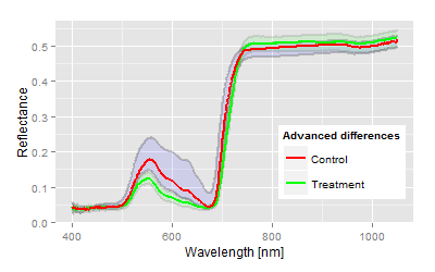
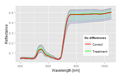
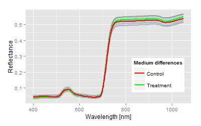
We have chosen one top and bottom end example to demonstrate the analysis of a two means comparison problem, somehow equivalent to a t-test (if you ignore the assumptions of a t-test). The graphs show the mean reflectance signatures of both control and treatment with the 95% confidence bands in the domain up to 1050 nm.

Visualisation: Spectral example for highly significant differences	Visualisation: Spectral example for no differences (n.s.)

After model fitting and discriminant analysis the result contains several statistical parameter (showing simultaneously in the same direction in most of the cases), which allow the interpretation of the trial. The interpretation must not be overstressed, the question in this case:
Is there a treatment effect compared to the control?
Nothing more and nothing less.

The table summarises the two examples depicted in the graphs above in terms of their gained statistical parameters, how these parameter changes with the situation, and what kind of interpretation exist.
Statistical parameter	Different	Explanation	No difference	Explanation
c²	P=0.000	The significance of the discriminant functions gives a first hint of treatment effects. As smaller the probability value p, as larger the differences	p=0.924	The usual boundaries are used: p>0.05 or better p>0.01, non significant (n.s.)
Canonical correlation	r=0.93	As in the classical correlation we can use the common separation: 0-0.3: no difference; (ns) 0.3-0.8: poor to medium differences, significant difference; 0.8 to 1.0, highly significant different; (***)	r=0.193	no correlation, not significant
Canonical distance	4.9	The most interesting parameter: Based on an arbitrary, dimensionless scale we can quantify the comparison, the value describes the intensity of the treatment effect.	0.4	Distance is less than 1, obvious no treatment effect.
Classification	95%	Very high percentage of correct classification, the data distribution indicates a large difference and a clear distinction.	50%	The bottom end of any classification; the result indicates randomness; no distinction possible; in fact no treatment was induced in this data set.

ANOVA of the mean comparison
		Difference		No difference		Explanation
Parameter	Model label	F-value	p-value	F-value	p-value	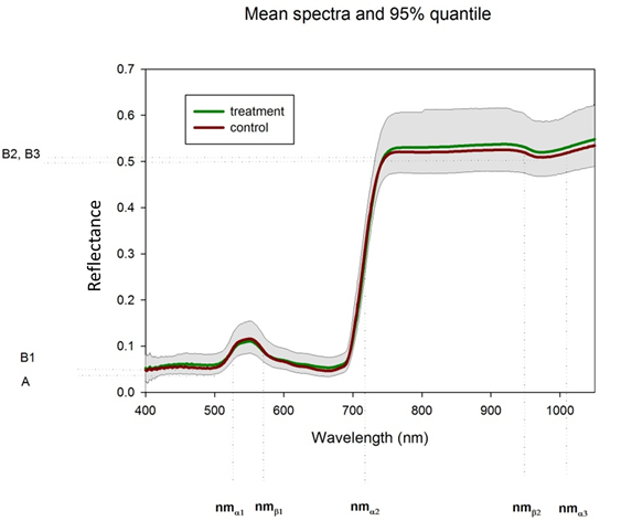Slight cut backs must be made in the interpretation of the ANOVA table, as the internal correlation of the model parameter is not taken into account in the ANOVA, therefore it should be used for orientation only. The standard boundary of 5% for the statistical decision is not valid here. We assume p-values <0.01 (or < 1%) are significant, certainty exists with p-values <0.000. The more the spectra differ, the more model parameters are significant different. In case of significances, the size of the F-value depicts how much of the distinction is affected by this parameter and in which domain of the spectra treatment effects are largest. The model exponents (not shown in the graph) are describing the slopes of the amplitudes, but should not get too much weight alone in the interpretation of the results.
A	A	0.821	0.371	0.097	0.756
B₁	B1	25.717	0.000	0.000	0.994
nm_a1	AC1	0.408	0.527	0.250	0.617
nm_b1	BC1	39.282	0.000	0.41	0.840
a₁	AL1	4.134	0.049	0.451	0.503
b₁	BE1	3.060	0.089	0.474	0.492
B₂	B2	16.369	0.000	0.008	0.930
nm_a2	AC2	62.845	0.000	0.011	0.920
nm_b2	BC2	37.501	0.000	0.003	0.054
a₂	AL2	37.778	0.000	0.041	0.839
b₂	BE2	4.856	0.034	0.198	0.657
B₂	B3	16.869	0.000	0.003	0.955
nm_a3	AC3	50.742	0.000	0.343	0.558
a₃	AL3	15.492	0.000	0.375	0.541

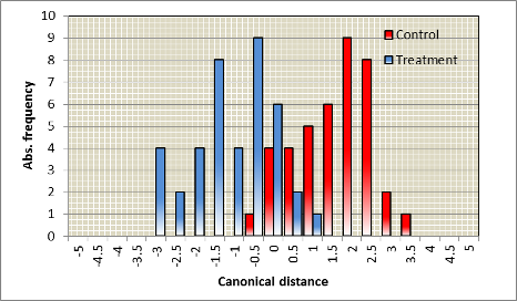
Summary classification
Distribution of classification (discriminant scores), different	Distribution of classification (discriminant scores), no difference

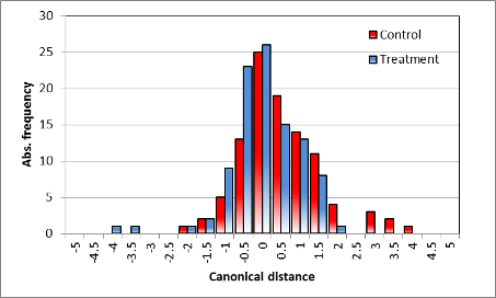Demonstration of the variance found in the spectral measurements, also affected by the individuality of the specific single plant. No overlapping exits in the distribution, but an obvious discrimination of the treatment.	Obvious overlapping of the distance classes, no distinction of the spectra, variance larger than the mean canonical distance.

A typical outcome of an experiment

On average data will be most likely in between the two extremes as the following example shows; the following spectra were recorded with given variance

Spectra	Distribution of discriminant scores

Statistical parameter	Value	Explanation
c²	P=0.000	Discriminant function is significant indicating a significant difference between treatment and control.
Canonical correlation	0.80	Correlation is high on a scale from 0 to +1, also for this parameter, the difference is obvious.
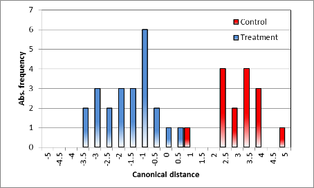
Canonical distance	2.74	The averaged distance is relatively high, overlapping classification scores are due to the natural variance by the individual plant.
Classification	90%	Extremely high for spectra apparently not differing from each other.

Model label	F-value	p-value	ANOVA table and explanation
A	0.331	0.567	By chance, the given example demonstrate the limits of the ANOVA. Numerous parameter are below a p-Value of 5%, but by the criteria to use here only parameter Bcrit2 and Acrit3 account for the differences caused by the treatment. Both parameter describes the amplitude in the higher wavelength domains. The treatment effect leads to changes in the structural tissue of the plant.
B1	0.072	0.790
AC1	2.858	0.095
BC1	4.041	0.048
AL1	4.962	0.029
BE1	6.362	0.014
B2	4.389	0.039
AC2	0.004	0.951
BC2	7.248	0.009
AL2	8.362	0.005
BE2	0.099	0.754
B3	4.478	0.038
AC3	30.832	0.000
AL3	1.173	0.282

Summary

The common example shown here demonstrates how reflectance data are used to discriminate simple treatment effects out of a cloud of information and how to confirm your findings in statistical terms. To address the individuality of your experiment, just the hyperspectral signature data are needed.

Testing for differences between two mean spectra and results:

Summary classification

A typical outcome of an experiment

Summary